Difference between revisions of "Ecological Modeling"
| Line 85: | Line 85: | ||
[[Image:PresenceData.jpg|frame|left|Figure 1.]] | [[Image:PresenceData.jpg|frame|left|Figure 1.]] | ||
| − | [[Image:SuitableMapManuallyReviewed.jpg|frame| | + | [[Image:SuitableMapManuallyReviewed.jpg|frame|left|Figure 2.]] |
[[Image:SuitableMapFromAquamaps.jpg|frame|left|Figure 3.]] | [[Image:SuitableMapFromAquamaps.jpg|frame|left|Figure 3.]] | ||
| Line 93: | Line 93: | ||
[[Image:CloseAbsenceData.jpg|frame|left|Figure 4.]] | [[Image:CloseAbsenceData.jpg|frame|left|Figure 4.]] | ||
| − | [[Image:SuitableMapFromNeuralNetwork.jpg|frame| | + | [[Image:SuitableMapFromNeuralNetwork.jpg|frame|left|Figure 5.]] |
We trained the network with all the presence and absence points. The best performing neural network had 1 inner layer with 100 neurons. The map produced by this system is depicted in figure 5 and presents a big spread in the ocean. The map superposes to the reviewed one, but it is quite far from the Aquamaps-Suitable distribution. The holes left by the neural network correspond mainly to low probability points in the reviewed map. Figure 6 depicts this superposition. | We trained the network with all the presence and absence points. The best performing neural network had 1 inner layer with 100 neurons. The map produced by this system is depicted in figure 5 and presents a big spread in the ocean. The map superposes to the reviewed one, but it is quite far from the Aquamaps-Suitable distribution. The holes left by the neural network correspond mainly to low probability points in the reviewed map. Figure 6 depicts this superposition. | ||
[[Image:NeuralNetwork1VSReviewed.jpg|frame|left|Figure 6.]] | [[Image:NeuralNetwork1VSReviewed.jpg|frame|left|Figure 6.]] | ||
| − | [[Image:RandomAbsenceData.jpg|frame| | + | [[Image:RandomAbsenceData.jpg|frame|left|Figure 7.]] |
The second experiment used absence data randomly chosen among the reviewed map points with low probability. Figure 7 depicts the absence data distribution. We trained again the neural network with all these points. This time the best performing presented 1 inner layer with 300 neurons. Figure 8 depicts the resulting distribution. As it can be noticed by the superposition map in 9, this time the distribution is close to the one from the Aquamaps algorithm instead of being similar to the reviewed map. | The second experiment used absence data randomly chosen among the reviewed map points with low probability. Figure 7 depicts the absence data distribution. We trained again the neural network with all these points. This time the best performing presented 1 inner layer with 300 neurons. Figure 8 depicts the resulting distribution. As it can be noticed by the superposition map in 9, this time the distribution is close to the one from the Aquamaps algorithm instead of being similar to the reviewed map. | ||
| − | |||
| − | |||
| − | |||
We tried to make some comments about this result: if we assume that the neural network is working correctly and it is able to learn something about the fish's attitude from the characteristics of the sea associated to the occurrence and absence points, this could indicate that the manually reviewed map could have been build on partial information about the fish. Furthermore this could mean that the reviewer performed the same considerations of the neural network. On the other side, if we are certain that the reviewed map is correct, then we must admit that the information extracted from the sea is not sufficient to understand fish's preferred habitat. Notice that two automatic systems almost agree on a certain distribution for the fish, which is far from the reviewed one and this could indicate the possibility of an evaluation error in the reviewed map. This case could be helpful for implementing an alert for a biologist who wanted to manually revise a map. | We tried to make some comments about this result: if we assume that the neural network is working correctly and it is able to learn something about the fish's attitude from the characteristics of the sea associated to the occurrence and absence points, this could indicate that the manually reviewed map could have been build on partial information about the fish. Furthermore this could mean that the reviewer performed the same considerations of the neural network. On the other side, if we are certain that the reviewed map is correct, then we must admit that the information extracted from the sea is not sufficient to understand fish's preferred habitat. Notice that two automatic systems almost agree on a certain distribution for the fish, which is far from the reviewed one and this could indicate the possibility of an evaluation error in the reviewed map. This case could be helpful for implementing an alert for a biologist who wanted to manually revise a map. | ||
| Line 115: | Line 112: | ||
*numeric comparisons were made in order to calculate the performances of the distributions. | *numeric comparisons were made in order to calculate the performances of the distributions. | ||
| + | [[Image:NeuralNetworkRandomAbsence.jpg|frame|left|Figure 8.]] | ||
| + | [[Image:NeuralNetwork2VSReviewed.jpg|frame|right|Figure 9.]] | ||
''Numeric details'': Experiments were performed considering as "correct positive classifications" probabilities higher than 80% and as "correct negative classifications" probabilities lower than 0.3 | ''Numeric details'': Experiments were performed considering as "correct positive classifications" probabilities higher than 80% and as "correct negative classifications" probabilities lower than 0.3 | ||
Revision as of 19:41, 15 February 2012
Ecological Modeling is a set of functionalities available in gCube for performing data mining operations on biological data. It is available as a library and as a Service (Statistical Manager) in the infrastructure and is able to train models which can be combined with geographical information in order to produce projections on several environmental scenarios or time periods. This system allows for managing complex phenomena, in order, for example, to predict the impact of climate changes on biodiversity, prevent the spread of invasive species, identify geographical and ecological aspects of disease transmission, help in conservation planning, guide field surveys, among many other uses.
Contents
Overview
The library is endowed with a set of features which can be resumed as:
- GENERATORS: include probability distributions, classifications, matching or distance measurements etc.
- MODELING: includes models to be trained, e.g. neural networks, species envelopes, support vector machines etc.. The result will be typically a binary file.
- CLUSTERING: involves clustering procedures for grouping together phenomena or multidimensional points.
- TRANSDUCERS: involve algorithms for transforming a dataset into another.
- EVALUATORS: a set of procedures for measuring the quality of a model.
The system is currently able to run processes on the following computational platforms:
- LOCAL MULTICORE MACHINE
- RAINY CLOUD
Generative Algorithms
Currently the following algorithms are supported for projecting probability distributions on geographical maps:
- AQUAMAPS_SUITABLE: Aquamaps Suitable habitat production
- AQUAMAPS_NATIVE: Aquamaps Native habitat production
- AQUAMAPS_NATIVE_2050: Aquamaps Native for 2050 scenario
- AQUAMAPS_SUITABLE_2050: Aquamaps Suitable for 2050 scenario
- REMOTE_AQUAMAPS_SUITABLE: Aquamaps Suitable habitat generated by invoking Rainy Cloud
- REMOTE_AQUAMAPS_SUITABLE_2050: Aquamaps Suitable 2050 habitat generated by invoking Rainy Cloud
- AQUAMAPS_NATIVE_NEURALNETWORK: Aquamaps Native Distribution using a Feed-Forward Neural Network
- AQUAMAPS_SUITABLE_NEURALNETWORK: Aquamaps Suitable Distribution using a feed-Forward Neural Network
- AQUAMAPS_NEURAL_NETWORK_NS: Aquamaps Suitable Distribution using a Feed-Forward Neural Network provided by Neurosolutions (http://www.neurosolutions.com/)
The above algorithms are automatically managed by an underlying library (Ecological Engine) which takes care of the selection of the most proper computational infrastructure for running the generation algorithm.
Modelers
Currently the following models are supported for training purposes:
- HSPEN: Hspen model by Aquamaps
- AQUAMAPSNN: Feed-Forward Neural Network for usage in Aquamaps generations
- AQUAMAPSNNNS: Feed-Forward Neural Network by Neurosolutions (http://www.neurosolutions.com/) for usage in Aquamaps generations
Even in this case, the above algorithms are automatically managed by the Ecological Engine library which takes care of the selection of a computational infrastructure suited for running the modeling algorithm.
Clustering
No clustering algorithms are currently available.
Transducers
No transducers are currently available.
Evaluators
Available evaluation techniques are the following:
- CLASSIFICATION QUALITY ANALYSIS: This evaluation method applies to a probability distribution and a set of occurrences\absence points. Calculation includes the following values
- TRUE_POSITIVES
- FALSE_NEGATIVES
- TRUE_NEGATIVES
- FALSE_POSITIVES
- ACCURACY
- SENSITIVITY
- SPECIFICITY
- DISCREPANCY ANALYSIS - BETWEEN TWO SPATIAL DISTRIBUTIONS: Evaluates the distance between two spatial probabilities distributions with the same resolution, in terms of
- ACCURACY
- MEAN ERROR
- VARIANCE
- NUMBER_OF_ERRORS
- MAXIMUM_ERROR
- MAXIMUM_ERROR_POINT
- NUMBER_OF_COMPARISONS
Experiments
Manual Review vs. Automatic Reviews
An experiment was performed using the Statistical Service. We tried to compare some Aquamaps distributions, automatically and manually generated, using a test case species (the basking shark): we selected a species for which we had availability of
- a good number of occurrence points
- a manually reviewed map
- a hspec-suitable map generated by the Aquamaps algorithm
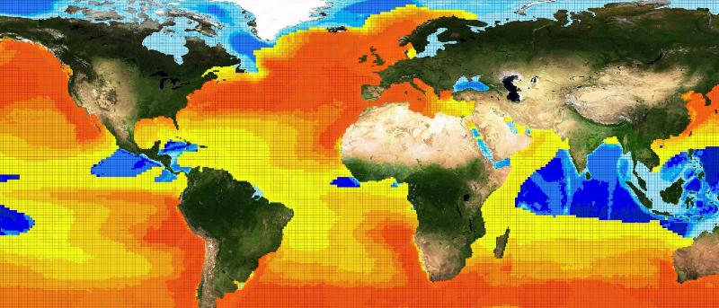
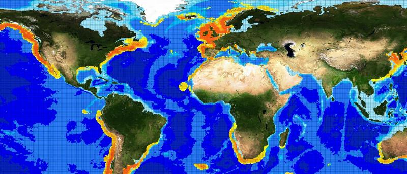
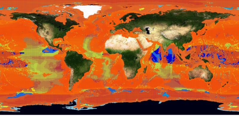
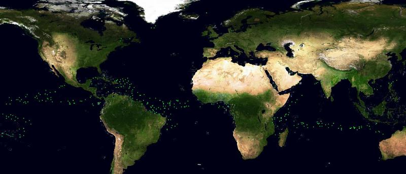
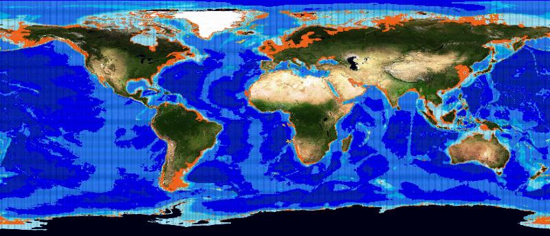
The choice fell on the Basking Shark species (Cetorhinus Maximus, Fis-22747). 449 presence data were available for this species. Figure 1 depicts the presence data distribution. Figure 2 depicts the manually reviewed distribution. Figure 3 depicts the original distribution produced by the Aquamaps-Suitable algorithm.
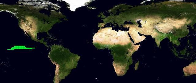
We tried to perform 2 experiments to test if an automatic machine learning system would have been able to extract species environmental preferences from the same parameters used by the Aquamaps algorithm. The machine learning system was trained with both presence and absence data: absence points were extracted from the reviewed map, from places with probability less than 0.1. We chose a feed forward neural network as machine learning tool, and the parameters we used for the training were the same as in the Aquamaps algorithm: depth mean,depth max,depth min,sst mean,sbt mean,salinity mean,salinity b mean, primary production mean,ice concentration,distance from land,ocean area. The first experiment used 449 absence data all coming from the same region where the reviewed map reported probability values less than 0.1. Figure 4 depicts this absence data distribution.
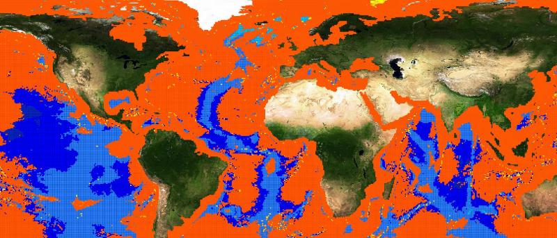
We trained the network with all the presence and absence points. The best performing neural network had 1 inner layer with 100 neurons. The map produced by this system is depicted in figure 5 and presents a big spread in the ocean. The map superposes to the reviewed one, but it is quite far from the Aquamaps-Suitable distribution. The holes left by the neural network correspond mainly to low probability points in the reviewed map. Figure 6 depicts this superposition.
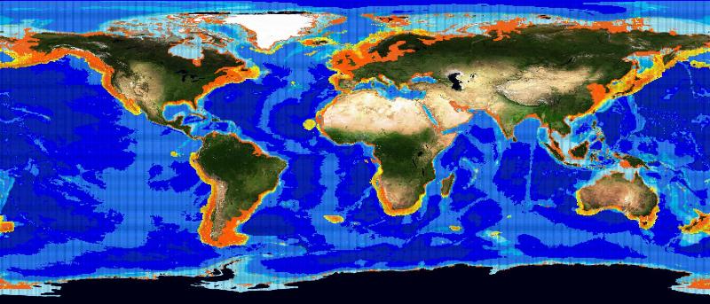
The second experiment used absence data randomly chosen among the reviewed map points with low probability. Figure 7 depicts the absence data distribution. We trained again the neural network with all these points. This time the best performing presented 1 inner layer with 300 neurons. Figure 8 depicts the resulting distribution. As it can be noticed by the superposition map in 9, this time the distribution is close to the one from the Aquamaps algorithm instead of being similar to the reviewed map.
We tried to make some comments about this result: if we assume that the neural network is working correctly and it is able to learn something about the fish's attitude from the characteristics of the sea associated to the occurrence and absence points, this could indicate that the manually reviewed map could have been build on partial information about the fish. Furthermore this could mean that the reviewer performed the same considerations of the neural network. On the other side, if we are certain that the reviewed map is correct, then we must admit that the information extracted from the sea is not sufficient to understand fish's preferred habitat. Notice that two automatic systems almost agree on a certain distribution for the fish, which is far from the reviewed one and this could indicate the possibility of an evaluation error in the reviewed map. This case could be helpful for implementing an alert for a biologist who wanted to manually revise a map.
Some final Notes:
- for the basking shark species all the maps are very similar either in the native or in the suitable distribution
- the neural network was trained many times with different topologies, in order to use the best configuration in each experiment
- the neural network does not need expert knowledge to produce the map from the inputs, but absence data are necessary, which come essentially from expert knowledge. This is a little paradox as neural networks are declared in literature among the best performing systems for producing distribution maps. Anyway the inputs are dependent on human knowledge.
- the values reported below refer to a training session using 449 presence and 449 absence data. Experiments were made even using 80% of the set for training and 20% for testing and were repeated using 60% for training and 40% for testing. The above considerations still remained valid.
- numeric comparisons were made in order to calculate the performances of the distributions.
Numeric details: Experiments were performed considering as "correct positive classifications" probabilities higher than 80% and as "correct negative classifications" probabilities lower than 0.3
Reviewed Map Performances on Occurrence Points
- TRUE_POSITIVES:332
- FALSE_NEGATIVES:117
- TRUE_NEGATIVES:449
- FALSE_POSITIVES:0
- ACCURACY:0.87
- SENSITIVITY:0.74
- SPECIFICITY:1.0
Aquamaps-Suitable Performances on Occurrence Points
- TRUE_POSITIVES:116
- FALSE_NEGATIVES:333
- TRUE_NEGATIVES:444
- FALSE_POSITIVES:5
- ACCURACY:0.62
- SENSITIVITY:0.26
- SPECIFICITY:0.99
Neural Network with 1 inner layers with 100 neurons - Trained on Dense Absence Data
- TRUE_POSITIVES:431
- FALSE_NEGATIVES:18
- TRUE_NEGATIVES:147
- FALSE_POSITIVES:302
- ACCURACY:0.64
- SENSITIVITY:0.96
- SPECIFICITY:0.33
Neural Network with 1 inner layers with 300 neurons - Trained on Sparse Absence Data
- TRUE_POSITIVES:218
- FALSE_NEGATIVES:231
- TRUE_NEGATIVES:428
- FALSE_POSITIVES:21
- ACCURACY:0.72
- SENSITIVITY:0.49
- SPECIFICITY:0.95
Calculation of the distance between distributions by point-to-point differences with tolerance 0.1
Distance of Aquamaps Suitable from Reviewed Map
- ACCURACY:92.04
- MEAN ERROR:0.46
- VARIANCE:0.053
- NUMBER_OF_ERRORS:8059
- MAXIMUM_ERROR:0.9
- MAXIMUM_ERROR_POINT:7301:101:2
- NUMBER_OF_COMPARISONS:101370
Distance of NN Dense Absence Data from Reviewed Map
- ACCURACY:96.80
- MEAN ERROR:0.57
- VARIANCE:0.084
- NUMBER_OF_ERRORS:3241
- MAXIMUM_ERROR:0.999
- MAXIMUM_ERROR_POINT:7506:206:2
- NUMBER_OF_COMPARISONS:101370
Distance of NN Random Absence Data from Reviewed Map
- ACCURACY:66.75
- MEAN ERROR:0.57
- VARIANCE:0.069
- NUMBER_OF_ERRORS:47138
- MAXIMUM_ERROR:0.999
- MAXIMUM_ERROR_POINT:1116:228:2
- NUMBER_OF_COMPARISONS:141762
Distance of NN Dense Absence Data from Aquamaps Suitable
- ACCURACY:82.41
- MEAN ERROR:0.51
- VARIANCE:0.063
- NUMBER_OF_ERRORS:2309
- MAXIMUM_ERROR:0.9
- MAXIMUM_ERROR_POINT:1414:362:3
- NUMBER_OF_COMPARISONS:13127
Distance of NN Random Absence Data from Aquamaps Suitable
- ACCURACY:93.71
- MEAN ERROR:0.56
- VARIANCE:0.055
- NUMBER_OF_ERRORS:8921
- MAXIMUM_ERROR:0.9
- MAXIMUM_ERROR_POINT:7516:485:2
- NUMBER_OF_COMPARISONS:141762

